Chapter 1 — Defining the piping system and its engineering basis
Define the connected equipment and active paths
For a vessel-to-pump suction system, pressure available at the pump depends on vessel liquid level and surface pressure, connecting elevations, fluid condition and resistance along the active path. The line boundary on a drawing does not end these hydraulic relationships or the movement transmitted through equipment nozzles.
A valve's required function can be throttling, blocking during an operating change or specified isolation. Its name and nominal rating do not establish that function. Likewise, a temperature indication does not establish a protective response. Define these functions for the relevant configurations before selecting components or measurement and control arrangements.
Match fluid condition to the arrangement
A two-phase stream divided between parallel exchangers can deliver different liquid and vapor fractions to each exchanger. Liquid momentum and the resistance offered to vapor affect the split. Equal pipe sizes do not establish equal phase distribution. Evaluate the incoming approach, branch directions, elevations, resistances and which equipment paths operate together against the required phase distribution. Unequal mixtures can change exchanger pressure losses and heat-transfer duties. Exchanger and reboiler arrangements develops the physical alternatives.
Retain composition, contaminants and credible service changes in the materials basis. Cooling-water constituents can affect alloy choice; sour constituents require their particular materials and intervention provisions. Low-temperature conditions can introduce failure concerns absent in normal warm service. See materials and piping classes and hazardous and cleanliness-sensitive services.
Associate flow rate, phase, density and temperature with the condition in which they apply. Maximum flow need not occur at maximum temperature, and a stream can change phase within its operating envelope. Unrelated maxima can conceal the combination that governs equipment performance or pressure generation.
Include elevation in the pressure basis
Pressure in a connected stationary liquid increases with vertical depth and density. Horizontal route length does not add static head. A pressure indication at one elevation therefore does not establish pressure elsewhere in the system.
During filling or testing, a high-point gauge can conceal excessive low-point pressure. Test-liquid density changes both the pressure difference and the weight carried by supports. Test-boundary pressure limits and support and restraint decisions apply these constraints. Elevation alone establishes no permissible test pressure or component adequacy.
For flowing service, combine elevation with equipment pressure generation and resistance. Pump suction and duty evaluation also requires vessel level, surface pressure and the fluid condition.
Flowing loss begins with the bore and the fluid condition
Include both flowing resistance and elevation in the pump-suction pressure balance.
Carry the flowing loss into the suction and available-head evaluation. Use the actual vessel level, surface pressure and liquid vapor pressure.
The method here assumes a circular, fully filled pipe. It also assumes that density and viscosity remain constant along the evaluated length. It does not model changing-density gas flow, phase change, two-phase distribution, water hammer or a transient operating change.
When bore or conditions differ, evaluate separate segments. Adding their lengths while retaining one diameter can conceal the controlling loss.
Let be volumetric flow in cubic meters per second, the actual inside diameter in meters and mean velocity in meters per second. Continuity gives
where is density in kilograms per cubic meter and is dynamic viscosity in pascal-seconds. The kinematic viscosity is , in square meters per second.
Before using the first expression, divide flow stated in cubic meters per hour by 3600.
Nominal pipe size identifies a size series. Wall thickness and lining determine the bore. Using DN as the inside diameter changes velocity, Reynolds number and the loss calculation together.
The flow regime determines how a friction lookup may be used. Laminar flow is expected below Re 2300 and turbulent flow above Re 4000. Between them, the flow can switch regime and pressure loss can change by a factor of three or more.
Do not interpolate a single stable factor through this transition interval. Before treating a nominal factor as a repeatable pressure-loss prediction, resolve the operating regime and its consequences.
Roughness and factor convention travel with the lookup
A roughness chart supplies a material and diameter relation for the friction chart. Its nominal diameter index is a separate convention from in Reynolds number. For the historical chart basis illustrated here, the printed absolute roughness labels are:
- 50 μm for carbon steel/alloy;
- 120 μm for bitumen-lined pipe;
- 260 μm for cast iron;
- 1500 μm for cement-lined pipe.
A separate note gives 50 μm for smooth cement-lined pipe of DN 400 and larger. The cement categories therefore cannot be collapsed into one material permission. The labels do not characterize every new, corroded or fouled pipe of that material.
For the installed pipe, confirm the material, lining, surface condition and applicable roughness basis.
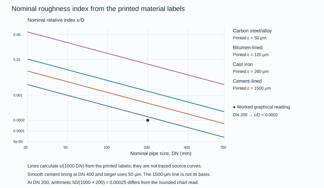
Figure 1.1. A reproducible arithmetic illustration of the nominal roughness index from selected printed labels. The lines use ε/(1000 DN), with ε in μm and DN in mm. They do not digitize every material curve.
The point preserves the worked graphical reading for DN 200 carbon steel/alloy. At that size the label arithmetic gives 0.00025, while the worked chart reading uses approximately 0.0002. Those levels of precision remain distinct.
For the worked graphical route, DN 200 carbon steel/alloy gives relative roughness approximately 0.0002. At Re 70,000 the stated friction reading is . A wider recovered lookup below supplies six solid roughness curves over approximately Re 50,000–50 million. Each saved curve has original graphical samples. The original dashed example projection is distinguished from the solid curve family.
The textual worked reading remains separate from a rounded trace reading. They are not forced to coincide exactly.
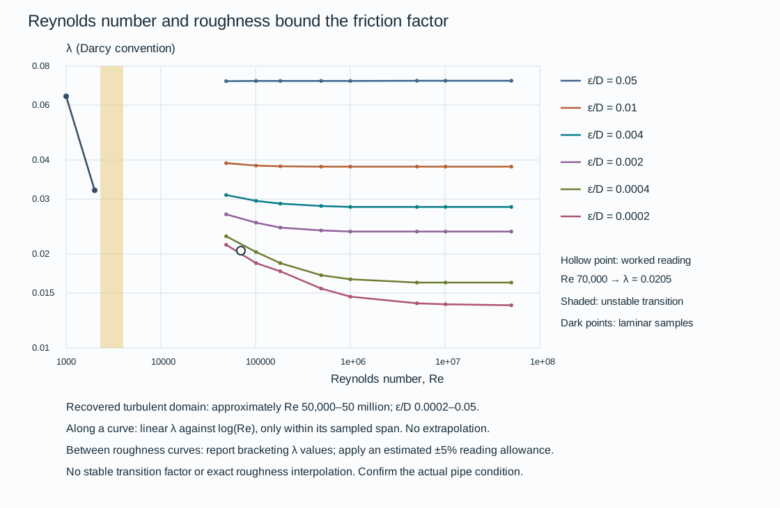
Figure 1.2. Approximate graphical recovery for relative roughness 0.0002, 0.0004, 0.002, 0.004, 0.01 and 0.05. Along each recovered curve, use straight joining of λ against log(Re) only between saved samples. For a roughness between two curves, report the two bounding factors instead of claiming an exact interpolation.
An author-estimated ±5% allowance expresses graphical reading resolution, not a statistical confidence bound or a design margin. No extrapolation or transition factor is supplied. Two laminar graphical points illustrate the separate regime.
For example, the nominal index from the cast-iron label at DN 100 is . At Re 100,000 that lies between the 0.002 and 0.004 curves, which give approximately λ 0.0252 and 0.0296. The lookup therefore supports a factor bracket, about 0.0239–0.0311 when the estimated graphical allowance is included.
The pressure-loss equation fixes the factor convention:
In these equations, is frictional pressure loss in pascals and is total equivalent length in meters. The quantity is loss in meters of the flowing liquid. The λ convention is the Darcy factor. If a calculation supplies a Fanning factor , the corresponding λ is .
Inserting directly into the displayed equation understates the loss by four. Before transferring a factor from another representation, identify the convention from the equation and accompanying data.
Equivalent length belongs to the selected component state
For the adopted procedure, total equivalent length is straight-pipe length plus the equivalent lengths of fittings and fully open valves on the active path.
The table uses nominal diameter , expressed in meters when calculating . The loss equation retains the actual bore . Selected entries illustrate the distinction:
| Component and state |
Equivalent length |
| Fully open gate valve, standard bore |
|
| Fully open ball valve, reduced bore, DN 40 and smaller |
|
| Fully open ball valve, reduced bore, DN 50 and larger |
|
| Equal tee, flow straight through |
|
| Equal tee, flow through side outlet |
|
| 90° elbow, radius |
|
| 45° elbow, radius |
|
The complete structured equivalent-length table preserves the remaining component patterns and size conditions. These values belong to this adopted procedure. An inline instrument or equipment item needs its own manufacturer loss data.
Use manufacturer data for critical losses. Avoid counting a loss through both an equivalent length and a separate pressure-loss term.
The fully open valve entries do not describe a partially closed valve. A changed component position or a dirty strainer can invalidate the loss basis even while nominal pipe size remains unchanged.
A preliminary liquid lookup narrows the alternatives
The flow–velocity relation can compare candidate bores before a final pressure-loss evaluation. The native plot below uses a selected printed schedule basis. It uses DN 50, 80, 100 and 150 in Schedule 40, and DN 200 in Schedule 30. Its inside diameters are respectively 52.48, 77.92, 102.30, 154.10 and 205.0 mm.
At 100 m³/h, for example, the 154.10-mm bore gives approximately 1.49 m/s. The 205.0-mm bore gives approximately 0.842 m/s. Before transferring either result to a system calculation, select the actual pipe wall and lining.

Figure 1.3. Calculated continuity relationships for explicitly stated printed bores, with flow in m³/h and velocity in m/s. The structured dimensions, graphical readings and worked calculation, and reproducible drawing implementation, preserve the distinctions between tabulated dimensions, recovered chart readings and hypothetical inputs.
One preliminary liquid-sizing procedure presents three flow panels: 0.1–10, 10–1000 and 1000–10,000 m³/h. Its suction and discharge areas use water at 20°C and pressure loss per 100 m: 0.034–0.083 bar for suction and 0.149–0.627 bar for discharge. These are pressure-gradient bands, not pump inlet or discharge pressures.
Within that procedure, more than one size can lie in the indicated area. In that case, the smaller size is selected for lines up to 100 m and the larger for longer lines. The local procedure is not a universal size selection rule. Preserve it with its water basis.
The preliminary interconnecting-liquid velocity band is 0.5–5 m/s in this basis. It excludes sludge, slurry, erosive fluids and two-phase flow. Being inside the band does not establish final acceptability. Under the adopted project conditions, evaluation is still needed for:
- Allowable pressure loss;
- Surge, erosion and vibration;
- Solids settling and viscosity changes;
- Mechanical strength and the equipment duty.
The related carbon-steel water-loss charts cover 1–10, 10–300 and 300–10,000 m³/h. Their first panel is headed 2°C. The continuation panels are headed 20°C. The discrepancy prevents treating the three panels as a single calibrated temperature basis. The middle-panel readings below remain attached to its 20°C heading. No temperature correction or whole-range join is supplied.
The charts identify DN curves, but do not state their bore and roughness numerically. Dimensions from the separate continuity table cannot establish those hidden chart inputs.

Figure 1.4. Recovered middle-panel DN 100, 150 and 200 curves. Samples include intersections with the stated preliminary suction and discharge gradient bands. Straight joins in log(flow)–log(gradient) space provide a bounded graphical lookup within each curve's saved span. They do not fit a physical loss equation or reveal the unstated bore. No extrapolation, interpolation between nominal sizes or first/third-panel join is supplied. The plotted bars express an author-estimated ±15% pressure-gradient reading allowance, not acceptance tolerances.
As a worked graphical comparison, take 130 m³/h on that middle panel. The recovered gradients are approximately 1.63 bar per 100 m for DN 100, 0.211 for DN 150 and 0.0497 for DN 200. Including the estimated reading allowance gives about 1.39–1.88, 0.180–0.243 and 0.0422–0.0572 bar per 100 m respectively.
The DN 100 result is above both preliminary bands. DN 150 lies within the adopted discharge band and DN 200 within its suction band.
This comparison is conditional on the chart's carbon-steel-water basis and shows which alternatives merit further evaluation. It does not select a final size for another liquid or establish available suction head. A nominal straight-pipe gradient multiplied by actual straight length does not include component, instrument or equipment losses. Those losses are included only if their adopted representations are added separately.
Changing the flow at a retained DN is a different operation from comparing DNs at one flow. On the recovered DN 150 curve, about 58.8 m³/h corresponds to 0.050 bar per 100 m. About 157.7 m³/h corresponds to 0.300 bar per 100 m. This sensitivity is visible in the recovered data rather than inferred from a single fixed-gradient slice. Keep the graph's approximate precision when interpolating between these samples.
The separate actual-bore continuity plot can calculate velocity after the wall and lining are selected. Its printed bore dimensions are not assigned to the pressure-chart curves.
Where temperature, chart dimensions or surface condition remains unconfirmed, the chart can explain the relationship without supporting a final size decision. A change in service, wall thickness, lining or configuration reopens the corresponding calculation inputs.
Steam hydraulic lookups retain the selected state
A steam pressure-loss lookup describes a flowing vapor at a stated condition. Pressure, temperature, phase, mass flow and nominal size belong together. A mass rate in kilograms per hour is not an actual volumetric rate. With a separately established density in kg/m³, gives m³/s when is in kg/s. Before that calculation, divide kg/h by 3600.
An actual-bore velocity calculation then uses . Neither nominal size alone nor a pressure label establishes density or velocity.
Four fixed-state chart bases are kept separate here:
| Phase label |
Pressure, bar gauge |
Temperature, °C |
| Dry saturated steam |
3.5 |
150 |
| Superheated steam |
13 |
270 |
| Superheated steam |
18 |
350 |
| Superheated steam |
44 |
440 |
The paired values and phase labels identify the chart conditions. They do not replace a property calculation. For properties or a pressure-loss fraction, establish absolute pressure as using the relevant atmospheric reference. Do not enter 13 bar gauge as 13 bar absolute into a steam-property relation. Do not infer density from gauge pressure alone. Confirm the actual pressure, temperature and dry-vapor state independently, including whether cooling or expansion produces condensate.

Figure 1.5. Approximate graphical recovery for DN 100, 150 and 200 in four separately labeled steam states. Each curve has a saved mass-flow span, so a lower or higher flow on another state's curve cannot be obtained by extrapolation. Straight joins in log(mass flow)–log(gradient) space approximate the original trace between recovered samples only. An author-estimated ±15% pressure-gradient allowance expresses graphical reading resolution, not a design margin or statistical confidence interval.
The original fixed-state charts also contain thick historical allowable-pressure-drop envelopes. Those envelopes are not reconstructed or adopted here. Recovered hydraulic readings can lie outside them. A point on a displayed curve therefore supplies no source-sizing admissibility or size-selection permission.
These DN chart curves do not disclose numerical wall, bore or roughness inputs. A separate bore table is not assigned to them.
At 5000 kg/h on the 13-bar-gauge, 270°C panel, the recovered DN 100 curve gives approximately 0.377 bar per 100 m. DN 150 gives approximately 0.0508 bar per 100 m. Their estimated reading ranges are about 0.321–0.434 and 0.0431–0.0584 bar per 100 m respectively. The comparison shows the influence of nominal size on the chart basis. It does not prove either size permissible. For this recovery the DN 200 curve begins above 10,000 kg/h, so no DN 200 result is supplied at 5000 kg/h.
A complete pressure-loss allowance must also address fittings, instruments, equipment and the actual path.
A density selector uses its own velocity baseline
For steam conditions outside the four fixed-state panels, a separate lookup uses density or its reciprocal, specific volume . Its two original density ranges are 100 down to 5 kg/m³ and 5 down to 0.1 kg/m³. The native recovery below retains the panels separately and uses only their saved DN-specific sample spans. The pressure gradient is based on 40 m/s, with a dimensionless correction
In these equations, and are gradients in the same unit, here bar per 100 m. Use matching velocity units in numerator and denominator. The correction factor is not an allowable velocity. The rounded table includes at 30 m/s and 2.25 at 60 m/s. Direct evaluation at 30 m/s gives 0.5625. Keep a literal rounded lookup distinct from the more precise equation evaluation.
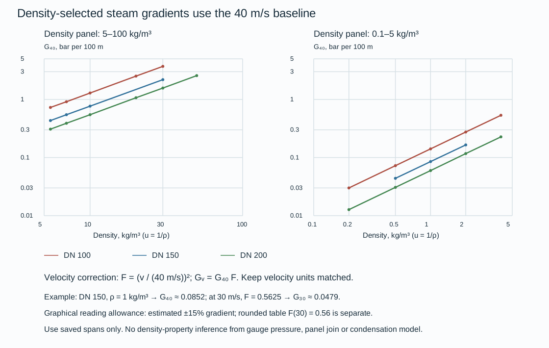
Figure 1.6. Selected density curves for DN 100, 150 and 200 at 40 m/s. Interpolation joins log(density) and log(gradient) within a saved curve span only. The two panels are not joined. State curves, recovered samples, correction table and worked inputs preserve the numerical conditions. The drawing implementation regenerates the native figures from saved data.
A steam line does not become constant-density merely because a chart supplies one point. Accurate gas and vapor pressure-loss evaluation needs a method that follows density, pressure, temperature and phase through the path. A bounded approximate procedure can use density and mean velocity at either inlet or outlet for a loss below 10% of upstream absolute pressure. A loss of 10–40% uses averages of inlet and outlet values.
Those conventions describe an approximate method where an accurate result is not required. They do not validate a large loss, a long cooling route, a choked condition or a two-phase calculation. At a larger or otherwise consequential change, use the appropriate compressible-flow/property calculation rather than extend this chart.
Condensate formation changes the physical problem. The dry-vapor curves cannot represent a flooded low point or flashing return. Steam and condensate behavior and thermal treatment provide the phase and heat-loss context. This hydraulic method supplies no distribution, consumer, trap or control arrangement.
Short gas lines can make acceleration part of the pressure loss
A short gas passage can change velocity enough that kinetic-energy change matters alongside wall friction. A liquid constant-density formula does not represent that mechanism. Conversely, a pressure-loss correlation suitable for a long pipeline does not automatically describe a short entrance-to-outlet passage. Before transferring numerical results, preserve the pressure stations, inside bore, length, mass flux and compressible-flow model.
A bounded dimensionless chart uses the abscissa
The chart uses the ordinate and a family parameter labeled . Here is mass flux, distinct from total mass rate, and is specific volume, distinct from velocity. The original customary-unit definitions give:
- in lb/(s·ft²);
- Pressures in lb/ft²;
- in ft³/lb;
- Pipe length and actual inside diameter in feet;
- .
The friction factor is not identified as Darcy or Fanning. The numerical gravity entry alone does not establish the legacy mass/force conversion convention.
The pressure stations introduce a further limitation. The diagram puts in the upstream reservoir, at the pipe entrance and at the outlet. The textual definitions call inlet pressure and do not define . Do not silently set or move an entrance loss into another station. Pressure ratios and property evaluations need compatible absolute pressures. Converting a gauge indication to absolute pressure does not resolve this station ambiguity.

Figure 1.7. Selected recovered solid curves labeled isothermal, , for printed values 0, 2, 4, 10 and 20. A separately recovered dotted curve is labeled at . The dotted label alone does not establish an adiabatic heat-transfer model.
Curves are recovered only over saved spans, chiefly outlet ratios 0.8–0.95. Straight joins interpolate along a saved curve. No interpolation between family parameters or extrapolation toward a critical endpoint is supplied. Estimated graphical reading allowances are ±0.015 in pressure ratio and ±0.005 in .
The printed critical-outlet relations can be compared on this same dimensionless basis:
For the multiplier is approximately 0.7715. With an explicitly assumed , the formula ratios are 0.150 and approximately 0.116. These lines mark the chart's critical-ratio relation. They do not supply a generic valve choked-flow rule or a relieving-capacity result. The sparse recovered family traces are not extended to intersect the critical lines.
At the same assumed , linear joining of the recovered solid samples gives . The samples give approximately 0.931. Their estimated ratio ranges are about 0.839–0.869 and 0.916–0.946, before accounting for uncertainty in the selected abscissa. This comparison shows how the chart changes outlet ratio at a held dimensionless input and a different labeled friction-length parameter. It does not convert a project length or mass rate into those parameters.
The saved chart data, literal station definitions and formula evaluations distinguish recovered points from equations and teaching assumptions. The drawing implementation reproduces the native chart.
For a dimensional project evaluation, stop at the missing model inputs. Establish:
- The pressure-station definitions;
- Compatible absolute pressure and specific-volume basis;
- Mass/force/gravity convention;
- The friction-factor convention used by the adopted compressible method.
Mass flux then belongs to actual flow area, not nominal pipe size. Selecting a convenient factor or assuming reservoir pressure equals pipe-entry pressure would manufacture a normalization the chart does not establish. This bounded dimensionless method explains the pressure-ratio comparison while preserving that limit. It provides no long-pipeline, valve or relief-sizing acceptance.
A condition is not the complete state
Evaluate conditions with the actual connected configuration, temporary restrictions and active contacts. Normal operation does not represent installation, testing or maintenance.
A line in service may be hot, filled and free to move at a selected support. During construction it may be empty, incompletely insulated and temporarily restrained. During a test it may contain a denser liquid, be isolated by temporary blinds and have a spring blocked. During maintenance a heavy valve or spool may be removed, leaving a different connected assembly. The same line identity can persist through all of these states. The relevant weight, pressure boundary and load paths can change.
Pressure and temperature need the same discipline. Operating conditions describe the intended process envelope. Upset conditions address identified departures. Design conditions provide the adopted basis for selecting and evaluating the pressure boundary. Component ratings and allowable quantities belong to the component and governing evaluation basis. They are not interchangeable with a measured operating value.
Test conditions describe the specified verification state. A successful observation at normal operating pressure does not establish the design envelope. A successful test of one isolated boundary does not establish every later operating configuration.
Retain the combinations and configurations that produce the pressure. In a system containing a pump, a changed inlet pressure contributes to its discharge condition. A normal flow configuration and a blocked path can impose different demands. A pressure-generating machine, an isolated liquid segment and a heated vessel need different explanations of how pressure can rise. Pressure design, relief and depressurization develops the protective basis and its applicable criteria. The first task is to make the relevant system and state visible, so that protection is evaluated for the right problem.
Regeneration, steam-out and decoking may impose temperatures and movements absent from normal production. Retain their participating equipment, temporary connections and affected envelope.
A practical state inventory can begin as a concise working table. Populate it with the actual activities and conditions relevant to the system. Do not assume every row below is mandatory for every installation.
Table 1.1. Relevant system states and evaluation consequences.
| State or activity |
What can change |
Consequence to carry into evaluation |
| Normal operation |
Flow, composition, level, pressure and temperature within the operating envelope |
Process performance, containment and equipment interfaces |
| Startup or shutdown |
Participating equipment, flow paths, filling/draining and relative temperatures |
Temporary pressure, phase, movement and operating arrangements |
| Defined special service |
Regeneration, steam-out or maintenance-related connections and temperatures |
A different thermal or process envelope from normal production |
| Installation |
Connected equipment, empty weight, insulation and temporary restrictions |
Construction stability, fit-up and intended final geometry |
| Pressure testing |
Fluid density, boundary, blinds and support/restraint configuration |
Head, weight and reactions in the actual test state |
| Maintenance or repair |
Isolation, contents, removed items and temporary support |
Safe intervention and support of the remaining assembly |
| Modification or changed service |
Components, fluid, pressure/temperature, routing or restraints |
Reopening the assumptions and neighboring interfaces affected by change |
The model represents a selected system state
A mechanical model can retain a weight support after the pipe has lifted clear of it. That model contains a load path absent in that operating state. A pressure test carried out with temporary boundaries does not represent the final flow path until restoration is complete. A drawing showing a clear maintenance space does not ensure that later field-run piping leaves the space clear. These are differences between representation and installed reality. A more precise calculation alone cannot repair them.
The model must represent contents, temperature, connected equipment, imposed movements and active restraints or contacts under the applicable evaluation criteria.
More than one load case may be needed to evaluate a state. Different physical evaluations may examine the same state for different reasons. A hydraulic check, a pipe-stress calculation and a structural reaction check are related evidence. One passing result does not automatically satisfy the others.
Compare installed geometry, settings and movement freedoms with the evaluated configuration. A change in fluid condition, movement or contact reopens the affected model inputs.
Keep what is known distinct from what is chosen
The test-boundary pressure example separates assumed component limits from the elevation calculation. Its 12 m height difference and liquid density determine the pressure difference. The assumed top-point minimum and low-point maximum then constrain the permissible gauge setting.
Whether that pressure is acceptable requires the applicable boundary, material, component and evaluation criteria. Changing the height or density changes the result. Changing an allowable changes the decision about the result. Neither change should be hidden by calling both quantities the design basis.
Criteria also need an application. Plant process piping, pipeline systems, boiler-related piping and offshore interfaces can have different governing boundaries. Establish the applicable codes, editions, jurisdictional requirements, project specifications and equipment limits for the actual undertaking. Historical references to ASME or API explain an engineering route where relevant. They do not establish present compliance. Buried piping, pipelines and offshore interfaces preserves the distinct system boundaries, and the specialist chapters carry the local criteria that influence their choices.
An unconfirmed vendor removal dimension prevents fixing the withdrawal envelope. A missing allowable prevents an adequacy conclusion. Preliminary arrangements can proceed only within the consequences of those unresolved inputs.
Compare solutions through the interfaces they change
The shortest or simplest-looking route is not necessarily the best system. A short hot pump suction line may reduce flow resistance while remaining mechanically stiff. Adding length and elbows can increase flexibility but also increase pressure loss. If a larger diameter is proposed to reduce that loss, its changed mechanical behavior has to be reevaluated. Hydraulic and mechanical choices interact. The first accepted calculation is not permanently fixed.
The same reasoning applies to access and construction. A compact equipment connection can use fewer fittings yet leave no practical spool for erection adjustment or component removal. An arrangement with deliberate break-out space may cost more initially but reduce recurring maintenance work. A dike or structure can perform its immediate function while constraining access, drainage or a piping route. Compare the complete arrangement across the states and tasks that give these features their purpose. Plant arrangement, access and constructibility develops the spatial method, and equipment and storage interfaces develops the particular physical requirements.
Compare diameter by annual capital and flow-energy cost
A pump or compressor can supply the energy needed to overcome flowing resistance. In that case, increasing the bore can exchange higher installed piping cost for lower machinery and energy cost. Compare feasible pipe sizes on a common annual basis. A line driven only by available pressure has a different selection problem. It must pass the duty within the available pressure and applicable limits. An economic minimum cannot create missing suction head, remove cavitation or make an incompatible material acceptable.
A customary-unit liquid correlation expresses annual comparable cost per foot as
In this equation, is chosen-currency dollars per foot per year. The variable is inside diameter in inches, and is US gallons per minute. The variable is liquid specific gravity relative to water at 60°F, and is a dimensionless Darcy friction factor. is total installed pipe cost per diameter-inch per foot, including the relevant painting, tracing and insulation. The variable is material plus direct field cost on that same basis. The variable is the indirect-field-cost fraction.
The symbol is a cost coefficient, not pipe length. is a simple before-tax payout period in years.
The variable is purchased machinery cost per hydraulic horsepower, and is its installation multiplier. The variable is comparable annual machinery and operating cost per hydraulic horsepower.
The load fraction is operating hours divided by 8760, with 80% entered as 0.80.
The electrical energy rate is in dollars per kWh, and combined pump/driver efficiency is a fraction. With those units, in dollars per hydraulic-horsepower-hour. An 80% efficiency is 0.80, not 80.
The correlation's numerical coefficient contains its customary units. To rounding, the coefficient is consistent with Darcy pressure loss and hydraulic power in horsepower for gpm and psi. It also uses water density near 62.4 lb/ft³.
Do not transplant that coefficient into an SI calculation. Before inserting a Fanning factor, apply its fourfold conversion. When viscosity, regime or duty changes, use the appropriate friction and machinery model.
If , costs and efficiency are held constant while considering continuous diameter, differentiating this objective gives
This is a continuous teaching optimum, not a purchasable nominal size. Its dependence on the cost ratio is weak. Doubling alone multiplies by . Doubling alone multiplies it by .
The relation is conditional on the constant-factor approximation. A revised bore can change Reynolds number and roughness ratio, requiring a new factor and cost comparison.
Equal length multiplying both diameter-dependent terms does not move this simplified optimum. Diameter-independent losses must still enter the complete hydraulic balance, even though they do not change this derivative.
Use actual installed and machinery costs, currency, tariff, demand charges, load fraction and efficiency. The dated correction-chart and machinery-cost inputs retained in the structured companion are not current estimates; its gas temperature convention needs confirmation before numerical use.
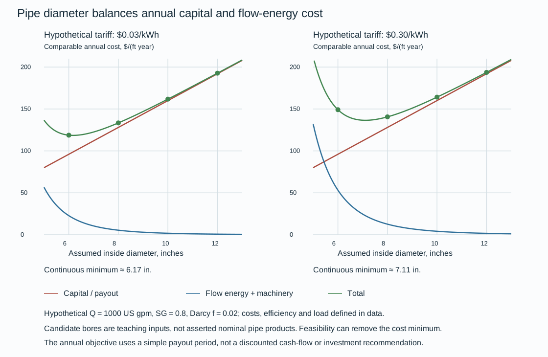
Figure 1.8. Hypothetical cost comparison at 1000 US gpm, , Darcy , dollars per diameter-inch per foot and a five-year payout. Machinery purchase cost is assumed 2000 dollars per hydraulic horsepower, installation multiplier 3, combined efficiency 0.75 and load fraction 0.80. The left and right energy rates are 0.03 and 0.30 dollars/kWh.
The candidate inside diameters 6, 8, 10 and 12 inches are teaching inputs. No particular nominal pipe product is asserted. The plotted annual objective is not discounted cash-flow analysis.
At the lower energy rate, the annual machinery/energy coefficient is about 1409 dollars per hydraulic horsepower per year. The 6- and 8-inch teaching bores give approximately 118.8 and 133.4 dollars per foot per year. Among the four candidates, 6 inches has the lower objective.
At the higher energy rate, rises to about 3290. Those candidates give approximately 149.1 and 140.6 dollars per foot per year, favoring 8 inches.
Continuous minima are approximately 6.17 and 7.11 inches. These results explain a cost sensitivity, not a recommendation for a real line. A pressure-loss constraint can eliminate the smaller candidate and leave a different feasible minimum.
Compare the complete valve assembly and its velocity reference
A smaller valve may save capital while adding flow-energy demand, reducer cost and installation space. For an installed assembly comparison:
- Include the valve, flanges and reducers.
- Use losses for the actual fully open flow path and the same physical coefficient reference.
An adopted dimensionless coefficient referenced to velocity in the valve bore gives the customary-unit liquid estimate
In these equations, is actual valve inside diameter in inches and is US gpm. The variable is liquid specific gravity and is hydraulic horsepower. The approximate expanded power expression is . Using keeps the pressure and power calculation internally consistent with the displayed rounded coefficient.
A coefficient based on upstream pipe velocity cannot be added directly to one based on valve-bore velocity. Convert both to one velocity reference or use validated whole-assembly pressure-loss data. Viscosity and other departures from this bounded liquid relation require the appropriate component method.
With installed assembly cost , the annual comparable cost is
In this equation, is dollars/year and is demand charge in dollars per kW-year. The variable is energy rate in dollars/kWh. Both efficiency and load are fractions. When demand cost is already included in the adopted tariff, set . Charging it again would double-count it.
The expression assumes the incremental machinery capital treatment embodied in the chosen comparison. Include a machinery or electrical upgrade when the added loss actually requires it.
For a bounded gas assembly relation, the corresponding customary-unit expressions are
In these expressions, is in lb/h, in lb/ft³ and in inches. Before entering a mass rate stated in thousand pounds per hour, multiply it by 1000. These local gas loss/power correlations do not replace a compressible-flow calculation when state changes are consequential. The expanded coefficient 19782 is rounded. No gas optimum is evaluated here without adopted state and assembly-loss data.

Figure 1.9. Hypothetical fully open assemblies with actual bore 6 inches and installed cost 6000 dollars, , or bore 8 inches and cost 10,000 dollars, . Both coefficients are assumed whole-assembly values referenced to valve-bore velocity. Other inputs are , five-year payout, efficiency 0.75, load 0.80, energy rate 0.10 dollars/kWh and demand charge 50 dollars/kW-year. These are teaching assumptions, not manufacturer data or product prices. Equation definitions, historical conditions, hypothetical inputs and calculated results keep the cost and loss bases recoverable.
At 1000 US gpm, the assumed assemblies lose about 0.543 and 0.0430 psi, yielding annual totals about 1436 and 2019 dollars respectively. At 2000 US gpm, their losses rise to about 2.17 and 0.172 psi and annual totals to about 3092 and 2150 dollars. The larger assembly becomes the lower-cost candidate. For fixed bore, coefficient and SG, doubling flow quadruples pressure loss and multiplies hydraulic power by eight. A changed operating fraction or efficiency also changes annual cost. Preserve those inputs with the state being compared.
Coefficient selection must precede a real comparison. The larger-size branch of a gate-valve relation is stated both as a constant 0.14 and as . This does not establish a unique coefficient for inches. Under its stated velocity and acceleration units, the enlargement expression gives time squared, rather than head in feet.
Neither ambiguity is used in the numerical examples. No corrected formula is silently substituted. Before evaluating those branches, obtain a validated loss relation or assembly data.
A piecewise enlarger relation with strict diameter ratios below and above 0.8 also leaves equality undefined. Its diameter/velocity reference must be established before combining coefficients.
The lowest annual objective is useful only among alternatives meeting the adopted hydraulic, NPSH, cavitation, pressure, erosion, phase, material and mechanical constraints. Reducers can affect stress and drainability. Larger hardware can affect support load, access and removal space. Evaluate discrete available products and the actual configuration, including credible changes in flow and duty. Pump suction conditions, pressure design, mechanical evaluation and access and constructibility can each remove a mathematically attractive candidate from the feasible set.
Carry the decision into installation, operation and change
Unconfirmed equipment envelopes may support plot alternatives without supporting final spool fabrication. Assumed liquid levels may support hydraulic sensitivity work without becoming operating data. Preserve the dimensions, component identities, settings and conditions on which the selected configuration depends.
Engineering records, human factors and lifecycle decisions develops the durable identities, revisions and work-system verification that connect these outputs.
A modification reopens the affected relationships. A replacement valve can change weight and removal space. A new temperature or fluid can change movement, density or material suitability. An added restraint intended to reduce vibration can oppose thermal movement. Changed operation can activate a previously unused flow path.
Reevaluate the neighboring components, states and calculations affected by a modification, retaining valid unrelated work.
Operating integrity and maintenance and repair and modification develop those interventions.