Chapter 10 — Flexibility, loads and vibration
Evaluate how the connected system responds
Weight support, pressure containment and displacement accommodation can compete: an offset can reduce thermal reactions while increasing weight deflection; a vibration restraint can increase displacement loads. Analyze the connected system.
The system description begins with pipe and component dimensions, materials, temperatures, contents, terminal connections and the support/restraint arrangement. Equipment can move. Structures can settle. Sliding contacts can resist movement or lose contact. The model represents those relationships.
It does not prove that the installed line has the represented gaps, freedoms, spring settings or boundary stiffness.
Before assembling load cases, define the physical states. An operating state combines contents, conditions, configuration and contacts. A test state can have heavier contents, different boundaries and temporary restrictions. A maintenance state can remove a component or terminal load path.
A load case evaluates a selected combination of inputs. Several cases can be needed to understand one state or the displacement range between states. The engineering basis and Support and restraint selection carry the corresponding system and installed-load-path account.
Separate sustained demand, displacement and dynamic forcing
Weight includes pipe, fittings, valves and operators, lining, insulation and contents. Test liquid belongs in the inventory even when normal contents are vapor. Concentrated mass at a valve can govern a span or nozzle moment differently from uniform weight. Snow and ice enter where required by the project. Pressure contributes to containment and mechanical loading. End thrust and pressure reactions need evaluation where the configuration produces them.
Sustained demand follows the load path available in the relevant state. A support that lifts clear of the pipe cannot continue carrying its assumed vertical reaction. A line can be acceptable while resting on every cold support. Its lifted hot configuration can have a different weight-stress problem. Separating thermal and weight calculations does not permit an impossible weight-support arrangement to remain in the model.
Thermal expansion, contraction, terminal motion and settlement impose displacement. Their effects depend on relative movement and restraint. Different demands arise from a uniform temperature rise between fixed points, a hot header with a cold standby branch, or an expanding vessel connected to a cooler line. Startup, shutdown, steam-out, decoking, regeneration and depressurization can produce other temperature combinations or ranges. Normal operation alone does not represent these. More than one analysis case may be needed to establish the relevant displacement stress range.
Wind, seismic effects and other occasional demands follow their adopted site and service basis. A particular project’s exemption from seismic calculation cannot become a general rule. Relief discharge, water hammer, slugging, machinery forces and pressure pulsation require their appropriate dynamic or transient treatment. They should not appear as unexplained additions to a normal static case.
Table 10.1. Physical states and mechanical evaluation consequences.
| Physical state or transition |
Inputs that change |
Evaluation consequence |
| Empty installation |
Incomplete insulation, disconnected equipment, locked springs or temporary supports |
Construction load path and fit-up may differ from the final operating model |
| Liquid test |
Fluid weight, temporary blinds, pressure and retained locks |
Test loads, temporary supports and terminal boundaries need the actual test configuration |
| Hot operation |
Metal temperature, sliding friction, lift-off and spring travel |
Sustained support path and displacement reactions must remain physically possible |
| Cold standby branch on a hot header |
Unequal temperatures and terminal conditions |
Relative branch/header movement can govern despite a satisfactory uniform-hot case |
| Steam-out or depressurization |
Temperature extremes, changing phase/pressure and equipment movement |
Review displacement range, material limits and connected equipment conditions |
| Maintenance or change |
Removed valve/spool, altered mass, new restraint or movement |
Reevaluate affected load paths and restore the intended configuration |
The cold endpoint is not always the installation temperature. The hot endpoint is not always the normal flowing condition. Sun can heat an idle line. A tracing or heating system can remain active after process flow stops. A vessel can be steamed while its connected line remains cooler. A dual-service line can experience both a hot fluid and a temperature below the winter ambient.
Establish the metal-temperature history and independently heated equipment, displacement interval and coincident pressure/contents.
One specifically adopted historical mechanical-analysis procedure illustrates this with a Celsius convention. It assumes a 50°C metal temperature from solar heating without flow and a −40°C winter endpoint. For a metal temperature above 50°C, it uses that temperature plus a 40°C interval. For a temperature between −40°C and 50°C, it uses a 90°C interval. Below −40°C, it uses 50°C minus the metal temperature.
These are conditional procedure temperatures; its paired Fahrenheit labels are rounded historical values. Use one consistent convention for absolute temperatures and intervals. A dual-service range can extend beyond these endpoints: use its full credible transition with applicable material growth data.
A real project must establish which endpoints and simultaneous equipment states are credible. A larger interval assembled from mutually impossible conditions is not automatically a better load case.
Calculate thermal growth from a defined reference
Thermal-growth data describe the change in length over a temperature interval for the selected material. A table of total expansion from a reference temperature is not a constant coefficient per degree.
Suppose is the tabulated growth, in inches, of a 100 ft reference length from a common reference temperature. The free growth of a straight length between temperatures and is:
Use in feet to obtain in inches for this table convention. The subtraction retains the common reference. Setting is valid only when is that reference. Negative tabulated growth represents contraction below it. Free growth is a displacement tendency. The actual restrained system develops forces and moments while accommodating growth through deformation and permitted motion.
The selected historical data below use 70°F as their reference. They illustrate material differences for preliminary understanding, with the grouping stated. They do not supply current qualified material properties for every grade or validate the material’s suitability at those temperatures.
Table 10.2. Bounded linear-growth reference values.
| Temperature, °F |
Carbon steel/C–Mo/low chrome through 3 Cr–Mo |
5 Cr–Mo through 9 Cr–Mo |
Austenitic stainless, 18 Cr–8 Ni |
| 70 |
0.00 |
0.00 |
0.00 |
| 200 |
0.99 |
0.94 |
1.46 |
| 300 |
1.82 |
1.71 |
2.61 |
| 400 |
2.70 |
2.50 |
3.80 |
| 500 |
3.62 |
3.35 |
5.01 |
Values are inches of linear growth per 100 ft between 70°F and the indicated temperature. Blank entries elsewhere in the underlying table are not zero properties.
Do not multiply a total-growth table entry by temperature rise; that counts the interval twice.
Resolve growth in the relevant directions between terminals and restraints. Add equipment or structure movement with its direction and sign. A nozzle moving toward the pipe’s free-growth direction can reduce one relative displacement and increase another. Settlement is imposed relative movement, with its own origin and time history. It is not a thermal expansion coefficient. Layout methods based on a stationary anchor must be revised when the terminal actually moves.
Offsets and loops turn growth into bending
A straight line between fixed ends has little geometric freedom to absorb axial growth. Bends, offsets and loops allow transverse legs to deform, reducing the reaction required to accommodate that growth. Their effect depends on the leg lengths, section stiffness, terminal constraints and component flexibility. A rigid valve or flange can shorten the effective absorbing length. An attachment near an elbow can reduce its assumed flexibility.
Choose a useful route before adding expansion devices. Direction changes required by the process arrangement can sometimes provide sufficient flexibility without a dedicated loop. A long header can distribute movement into flexible branches or direct growth from a selected fixed point. Those choices affect every connected branch and nozzle. A locally satisfactory offset therefore does not establish the entire header system.
Expansion joints provide another route when space or cost constrains pipe geometry. Bellows, sliding or other proprietary devices have particular movement, pressure-thrust, guide, anchor, fatigue and maintenance requirements. An axial joint can transfer pressure thrust to anchors. A flexible connector does not make that load disappear. If the adopted basis requires authorization for expansion joints, obtain it as part of selection. The device is not an ordinary substitute for an elbow.
The native figure defines the simple symmetric loop used in the next method. It shows geometric dimensions and anchor spacing. Weight supports, guides, bends and terminals still need their own design.
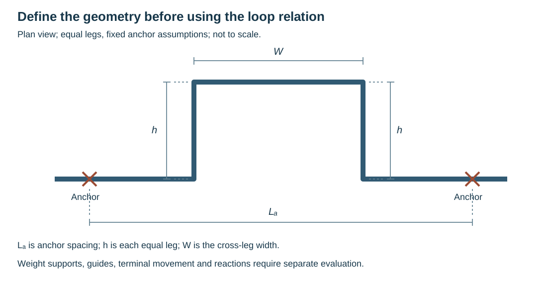
Figure 10.1. Plan geometry with equal legs , width and anchor spacing . The anchors are fixed assumptions of this preliminary method, not recommendations for every routed line.
A preliminary loop calculation needs its unit convention
For the historical standard-weight carbon-steel loop layout method shown, one preliminary depth relation is:
In this equation, and anchor spacing are in feet. Outside diameter is entered in inches, and temperature rise is in degrees Fahrenheit. The numerical constant embeds those units. It is not a dimensionless physical law that can be reused with millimeters, meters or degrees Celsius.
The same procedure applies a separate temperature-dependent minimum:
In this equation, is again entered in inches to obtain in feet. is the tabulated carbon-steel factor for the design temperature, distinct from the temperature rise. The procedure gives a minimum width and a preferred width . These are layout criteria for this method. They are not universal proportions or proof of acceptable anchor reactions.
The method’s standard-weight and material basis matters. A different section has different bending stiffness, and terminal motion can change the displacement to be absorbed. The historical quick-layout procedure supplies corrections for wall stiffness and anchor movement. Each correction requires its stated definition and geometry. Thicker pipe is not always mechanically better. It can increase the force needed to accommodate imposed movement.
L, Z and equal- or unequal-leg U configurations have different relations and leg checks, developed below. A numerical constant chosen for the symmetric loop cannot be assigned to any convenient offset. A fuller analysis needs the actual arrangement if route, component rigidity, support contact or terminal conditions differ materially from the simple method. Even a layout satisfying both loop checks still needs sustained-load, terminal-force/moment, pressure, local-detail and dynamic evaluations.
Choose the relation for the actual offset
An L-shaped route absorbs growth primarily by bending its shorter transverse leg. A Z-shaped offset provides two parallel legs of unequal length connected by that transverse leg. Equal and unequal U shapes distribute deformation through different leg arrangements. Their historical layout relations therefore use different coefficients and additional geometric checks. The letter describing the shape is not permission to use the symmetric-loop relation for it.

Figure 10.2. Schematics of fixed-end geometry, not to scale. In an unequal U, is the cross leg. In the equal U it labels each equal side leg. In the guided loop, and index the reaction/stress coefficients. Guides retain axial freedom. No weight-support or construction detail is specified.
For these quick-layout relations, use the following unit convention:
- Enter in inches.
- Enter leg lengths in feet and temperature rise in °F.
The standard-weight carbon-steel basis discussed above remains applicable. The procedure’s diameter convention rounds outside diameter upward to the specified half-inch increment. still corresponds to design temperature, not rise.
Pressure, branch/equipment restraint and special thermal conditions belong to the initial basis. Austenitic stainless steel and aluminum cannot inherit this carbon-steel basis merely by changing their names.
The L relation is , accompanied by . Its inverse maximum-long-leg expression is .
A Z uses the same growth-depth and inverse-length relations, but its parallel legs and must also satisfy , with . Both the transverse leg and the longer leg are tested against .
Equal parallel legs would fail this particular ratio condition even if the transverse depth passed. An apparently similar offset can therefore require a different evaluation.
For an equal-leg U, the relation becomes . Its inverse is . The independent evaluation is . is its cross-span as shown, not the developed length around both legs.
The unequal U uses the difference between the parallel legs. One printed relation is for . The further conditions are and . The reported alternative is not exactly the square root of that coefficient: , not 0.0021.
The discrepancy between the two printed depth forms remains a local method limitation. Do not silently average them or claim justified equivalence for a marginal arrangement.
More complicated planar routes can be decomposed into the major direction and the relevant transverse absorbing legs. The described planar adaptation compares the required short leg with the square root of the sum of squares of its specified perpendicular leg lengths. The three-plane adaptation first establishes the signed separations in each global direction and identifies the largest governing direction. These are geometry-specific adaptations. Summing every developed pipe length into one fictitious absorbing leg loses both direction and restraint information.
Section stiffness and terminal motion also change the quick-layout result. When wall differs from the standard-weight basis, the procedure adjusts minimum leg by . Where terminal expansion adds in that direction, it adjusts minimum leg by the ratio of total movement to pipe-leg movement. is the second moment of area, using equal length units in the ratio.
This is its stated correction, not a general scaling law for every bending problem. Signs and movement directions must be resolved before combining displacements. A beneficial terminal motion is not an unexplained reduction factor.
Resolve route legs before selecting an absorbing length
Figure 10.3 separates three geometric accounts. In the planar route, the signed horizontal separation is and the vertical separation is . The selected adaptation assumes the former is the major direction . It compares the required transverse length with . The negative sign on d describes its direction between terminals, while its squared length remains positive in that particular transverse comparison. Replacing both quantities by the sum of all pipe lengths would lose the distinction.
In the three-plane route, the terminal separations are , and . Before applying the selected adaptation, identify the largest separation in the actual geometry. The drawn example assumes governs. For that assumed direction, the transverse legs are b, c, d, f and g. The procedure compares their summed lengths with the required short leg. That is a different construction from the planar root-sum-square comparison, not a choice of whichever produces the smaller required route.
Retain the standard-weight, material, diameter, temperature and unit limits of the preliminary method above, including its unresolved alternative coefficient differences. Geometry alone supplies no stress or nozzle acceptance.
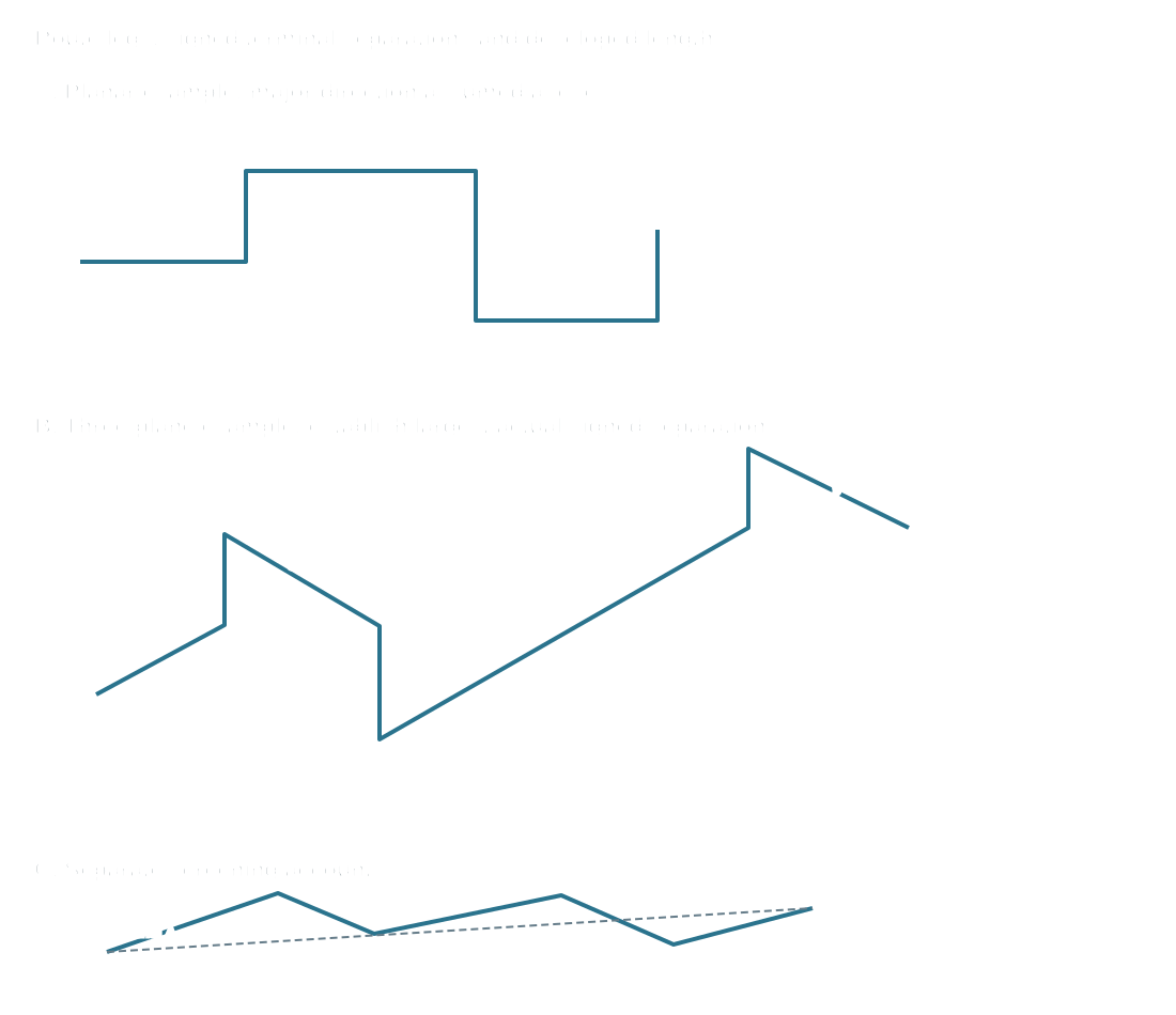
Figure 10.3. Schematic leg identifiers and signed directions. The third panel distinguishes developed pipe length from straight terminal separation . Neither is automatically the major-direction L or absorbing h used by an offset method. Structured geometry records the different accounts.
The separate screening procedure uses developed length and straight anchor separation as different inputs. A routed line with many turns can have a large developed length while its anchors remain close. Terminal movements must still be combined in their actual directions. A scalar chord does not turn several directional movements into one pipe-leg expansion. Each method needs its appropriate geometry. The symbol L must not be transferred between the sketch, a span table and a screening inequality.
A deliberate preset moves the cold and hot positions about a neutral datum
The neutral shape is the unstressed geometric datum for the illustrated L-route. Without a preset, the cold shape lies at that datum and heating moves the elbow in the expansion direction. A cold-spring preset deliberately positions the cold elbow on the opposite side. Heating then carries the elbow through the neutral position toward the hot position. Figure 10.4 distinguishes all four states. The specified amount, direction and fabrication sequence are part of the analyzed assembly, rather than an undocumented pull used to close a misaligned flange.
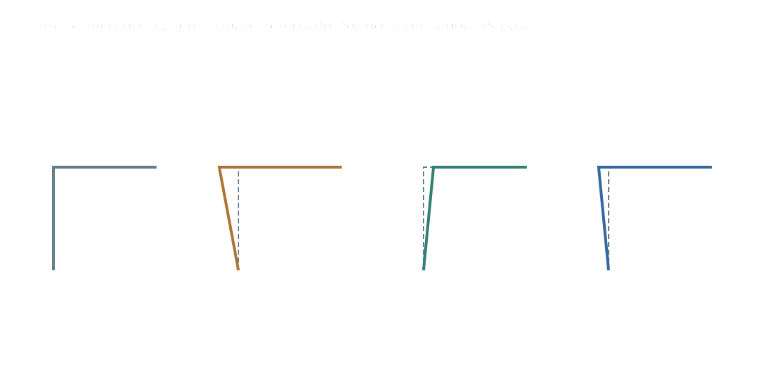
Figure 10.4. Conceptual positions relative to the same neutral datum. In a hypothetical one-direction example with 3 in growth and a 1.5 in opposing preset, the cold and hot offsets are −1.5 and +1.5 in. Without preset, the hot offset is +3 in. The drawn deflections are exaggerated and do not calculate force reduction. Structured state data retain the signs and assumptions.
The example redistributes cold/hot displacement about neutral. It does not reduce the thermal displacement range or establish a proportional reduction of every force, moment or stress. Actual supports, terminal movement, stiffness, installation tolerances and the authorized cold-spring treatment govern the result. A small prescribed amount can be lost within ordinary fabrication tolerance. When the analysis requires it, the drawing must specify an executable amount and hold tolerance.
Resolve any project prohibition or approval condition for cold spring at rotating equipment before specifying it. Installation verification and fit-up control carry that intent into construction. Force fitting is not a substitute for the analyzed preset.
Check what the loop sends to its anchors
Minimum layout depth answers whether the preliminary route has the prescribed geometric flexibility. It does not answer how much force each anchor receives or what maximum stress the loop develops. A separate guided-loop method addresses those questions for long-radius elbows and line sizes NPS 4 through 14. Expansion to be absorbed is limited to 10 in.
Its geometry includes equal loop legs , width , anchors outside the loop and guides on both straight approaches. The figure places each approach guide at least 40 pipe diameters from the associated loop bend. That historical layout condition is retained as stated. The diameter convention and actual guide detail must be established before applying it.
The relations are:
In these equations, is expansion to be absorbed in inches, not elastic modulus. is pipe second moment of area in in⁴. is outside diameter in inches. and are numerical coefficients indexed by and in feet.
In the method’s inch-pound convention, is force in lbf and stress is in psi. The corresponding coefficient dimensions are lbf/in⁵ for and psi/in² for . The tabulated numbers retain these embedded units; SI dimensions cannot be inserted into them. The force is the stated loop force at each anchor. It is not a complete six-component equipment-nozzle load vector.
The coefficient grids are identified by their actual and headings and their dimensions. The design-temperature grid serves the earlier minimum-leg evaluations. It cannot supply either reaction coefficient. The selected exact entries below avoid interpolation and illustrate the distinction between height and width effects.
Table 10.3. Conditional guided-loop reaction and stress coefficients.
| , ft |
, ft |
for force |
for maximum stress |
| 20 |
10 |
1.64 |
337 |
| 20 |
20 |
1.46 |
270 |
| 20 |
30 |
1.33 |
230 |
| 15 |
10 |
3.03 |
457 |
| 15 |
20 |
2.68 |
372 |
| 15 |
30 |
2.44 |
313 |
At fixed expansion and section, reducing loop height raises both demands in the displayed grid. Increasing width at fixed height lowers them, subject to the actual guides, weight support and available geometry.
These estimates do not establish allowable force, stress or fatigue life. The printed method does not provide a full derivation or every material/modulus, elbow or load-combination condition underlying its coefficient grids. The results are historical estimates within the displayed geometry/range. They require the applicable analysis and acceptance basis. Do not extrapolate to a different guide configuration or a table dimension outside its range.
A thicker wall can change and hence anchor force even when the same outside diameter is retained. The pipe-stress result must still be evaluated under its appropriate method and material basis. The existing equipment-load and model-contact account remains necessary alongside this useful preliminary calculation.
Keep force and stress inversions on their separate chart bases
A two-straightedge nomograph can invert a chosen planning criterion. For a directional thermal movement and pipe section, it estimates the absorbing leg required by that chart. Figure 10.5 preserves two different constructions.
The pump chart first joins expansion in inches to an assumed nozzle-force criterion in lbf, intersecting the pivot line. It then joins that pivot point to a section ordinate. The vessel chart first joins expansion to a stress criterion in psi, then joins the pivot point to nominal diameter. Each second line crosses its own pipe-length scale in feet.
A force and a stress are different physical quantities. Neither chart’s criterion can be moved to the other’s axis or combined with another method’s allowable.

Figure 10.5. Native reconstructed scales and two-line inversions within the recovered domains. The selected tick values retain original scale positions. Interpolation is logarithmic in the values between labeled ticks, while straightedge geometry is linear in chart coordinates. Source coordinates are graphic calibration, not pipe dimensions. Scale data, results and reproduction script preserve the bounded operation.
The pump chart's nominal-diameter marks are for standard-weight pipe. For another wall basis, the procedure uses its moment-of-inertia scale, in in⁴, instead of the nominal-diameter scale. Establish actual section inertia in the chart's units before making that substitution. The vessel chart has no recovered inertia axis here. It does not inherit the pump’s wall adjustment by analogy.
Both procedures depend on the selected route and the perpendicular legs available to absorb each directional movement, including terminal growth, stiff valves/nozzles and supports. A three-plane drawing is not permission to sum all unsigned growth into one displacement.
For preliminary pump planning only, the historical steel-nozzle assumption is lbf. The cast-iron assumption is lbf. Nominal nozzle size is in inches. These are author-selected planning criteria when published equipment data is unavailable. They are not code-defined or vendor-qualified loads.
The illustrative steel 10-in nozzle therefore gives 2,000 lbf. The line size used on the section axis can differ from the nozzle size used to select that force. The vessel example separately assumes 14,000 psi. It is not a complete vessel nozzle, shell or weld evaluation.
| Chart and declared inputs |
Approximate reconstructed length |
Graphical read band |
| Pump: 0.713 in, 2,000 lbf, standard-weight nominal 12 in pipe |
about 23 ft |
about 21.5–24.5 ft |
| Pump: 0.506 in, 2,000 lbf, same pipe |
about 20.5 ft |
about 19–22 ft |
| Vessel: 0.179 in, 14,000 psi, nominal 30 in pipe |
about 17 ft |
about 16–18.5 ft |
| Vessel: hypothetical 0.5 in, 14,000 psi, same diameter |
about 29 ft |
about 27–31 ft |
The first three input pairs follow the historical exemplars. The outputs here are independent graphical reconstructions with coarse read bands. The last pair is a hypothetical movement sensitivity comparison. The bands describe chart-reading/calibration uncertainty, not an engineering safety factor or statistical confidence. No underlying exact nomograph equation has been inferred. The saved reproduction rejects inputs or length outputs outside its recovered scales.
Near a comparison boundary, obtain a qualified analytical result. Additional digits in the graphical estimate do not resolve the comparison.
The bounded pump data cover expansion 0.2–2 in, force 1,000–3,000 lbf, standard-weight nominal sizes 10–24 in or inertia 200–2,000 in⁴, and length outputs 10–50 ft. The bounded vessel data cover expansion 0.1–2 in, stress 10,000–20,000 psi, nominal sizes 12–36 in and length outputs 10–70 ft. These are recovered graphical domains, not applicability limits that make every pipe/material in them acceptable. Each input must remain on its selected historical model and the actual engineering basis must supply current acceptance criteria.
The historical examples also contain two consequential ambiguities. One vessel step calls its east-west leg 18 ft while multiplying 25 ft. Its route drawing labels 25 ft. Those alternatives give different movements, so the stated example's result is not certified by silently selecting one.
Separately, a vertical-growth step multiplies feet by an inches-per-foot growth coefficient and prints 0.828 ft. The operation produces inches under that unit convention. The printed foot label cannot be adopted as a displacement without resolving the inconsistency. Preserve the entered length, unit and resulting direction together before using the chart. The native inversion data do not claim verification of those ambiguous example conclusions.
After a leg change, recalculate movements in all affected directions and the reactions at equipment and supports. Making one chart comparison favorable can increase another terminal's demand or alter access and weight support. Use this inversion as a bounded planning estimate with its declared criterion. The actual flexibility, nozzle/shell, attachment and structure assessment closes the design.
Screening identifies a need for deeper evaluation
A screening method is useful when its assumptions match the system and the result is treated as a bounded decision aid. Experienced comparison with a successful similar installation, a simple hand method and a detailed model have different evidential strength. Similar appearance is insufficient when temperature range, restraints, product stiffness or equipment limits differ.
One historical flexibility screen is:
In this inequality, is nominal pipe size entered in inches. is displacement to be absorbed entered in inches. is developed line-axis length in feet, and is the straight distance between anchors in feet.
This differs from outside diameter in the loop method. This differs from the loop’s anchor spacing. The threshold embeds the specified inch/foot convention. It is not a dimensionless acceptance value transferable to another unit system.
Source-specific analysis criteria can require formal evaluation independently of this screen. One adopted metallic-piping basis explicitly includes:
- Load-sensitive equipment
- Fired-heater and turbine lines
- Reciprocating equipment and relief systems
- Proprietary expansion devices
- Significant differential settlement
- Severe cyclic/vibrating service
- Jacketed piping and plastic-lined systems
Another uses different size and temperature triggers. For example, their centrifugal-pump triggers can be NPS 3 and larger under one basis and NPS 4 and larger horizontal-pump piping under another. Retain the applicable basis and its exceptions. Do not average the thresholds or use a favorable screen to evade a mandatory category.
Prepare signed relative movement before taking a resultant
The displacement supplied to a preliminary screen should be the movement that the connected pipe must accommodate. To prepare the displacement:
- Choose an origin and axes.
- Retain the signs of pipe growth and terminal movements.
- Before forming a magnitude, combine compatible components.
Taking the absolute value of each contribution too early can turn a movement that offsets another into an artificial addition. Conversely, adding a terminal motion as one unsigned scalar can hide an increased demand in a different direction.
A relative-displacement vector also has a reference condition. Equipment growth measured from a cold support datum must not be combined with pipe growth measured from a different, unexplained origin. Before using nozzle movement, resolve a segmented vessel temperature profile from its actual support reference. A nozzle’s elevation alone does not establish its growth. Rotation and settlement can require additional boundary inputs beyond this simple translation.
A resting support carries weight only while contact exists. A guide acts after its relevant gap closes. A stop limits selected travel. A spring changes load with travel according to its design. Rod hangers can swing and introduce horizontal reactions as their geometry changes. The pipe and support structure can both move, so a restraint relative to structure is not necessarily a fixed point in global space.
Sliding contact resists motion through friction. Its effect can redistribute force between supports and equipment, change which point moves and alter the path between cold and hot conditions. The model should reflect the adopted friction basis and actual surface/load arrangement. A frictionless assumption is a particular idealization, not the default meaning of “support.” Likewise, a perfectly rigid anchor can be an inappropriate representation of a flexible bracket, baseplate or structure.
One adopted analysis basis permits an assumption of frictionless unrestrained movement only for a system entirely supported by rod or spring hangers. It forbids adding friction to reduce calculated loads or stresses. That is a conservative modeling requirement under that basis. It does not mean that real hangers have no geometric reactions or that friction can never reduce a particular reaction physically. Keep the prescribed analytical treatment distinct from the mechanism and from other procedures.
Lift-off changes the sustained case. A procedure may require removing the lifted support from sustained calculations or considering a spring. That rule must apply to the relevant hot configuration. Simply leaving the cold reaction in the weight model while reporting lift-off in another case has not evaluated the available load path.
Attachments, refractory lining, thin wall and jacket/core interactions can require local or modified modeling. A lining can add weight and alter stiffness. An adopted procedure can include lining stiffness for displacement response. It can exclude beneficial stiffness in span/sustained evaluation to protect against creep effects. Pipe elements and default elbow/tee factors therefore need their applicable geometry and material basis. Detailed software output does not supply a missing local assumption.
Distinguish a stiffness representation from a local stress factor
An elbow absorbs displacement partly through deformation of its cross-section. A nearby attachment can interfere with that deformation, making the installed bend stiffer than a default bare-elbow element. A stress intensification factor modifies the stress evaluation for a local detail. It does not replace the element’s flexibility or the actual restraint. Revising one does not automatically revise the other correctly.
One specifically adopted historical ASME B31.3 metallic-piping analysis basis requires reduced flexibility to be represented for certain attachments. These are attachments on welded elbows or within two pipe diameters of an elbow weld. In the absence of better information, that basis permits a flange-pair representation at the nearest weld. It also specifies flange pairs at both ends of a 45° elbow.
These are analytical proxies within that basis. They do not specify installation of real flanges, qualify the attachment weld or supply its local allowable. Preserve the basis's diameter convention when establishing the proximity. The stated rule alone does not define nominal or outside diameter.
The same adopted basis provides separate stress-factor treatment for branch geometries outside its referenced default rules. For a branch at an angle other than 90°, applicable data or rigorous analysis may be absent. In that case, it permits twice the default stress intensification factor for an unreinforced fabricated tee. Its 3:4 tee aspect-ratio category requires a 25% increase.
These describe different geometric conditions. They are not alternative multipliers from which to choose the easier result. Establish which geometry and factor definition apply before using either, and do not infer an undefined aspect ratio merely from two nominal pipe sizes.
Carry these local choices into the system question. A stiffer bend can increase terminal reaction even when its stress-factor entry is unchanged. A higher stress factor can increase the reported local cyclic demand without producing a new physical restraint. The analysis record should therefore preserve actual attachment location, component geometry, applicable data or adopted proxy, and the resulting changes to both response and evaluation. The existing lining and lift-off distinctions likewise remain case dependent. No beneficial refractory stiffness is silently transferred into sustained or span assessment.
Pipe stress and equipment reactions have separate acceptance bases
A stress result describes an evaluated pipe demand under its code/method basis. A terminal force or moment describes the load delivered to equipment. The equipment can be sensitive to deformation, misalignment, casing stresses, footing forces or seal performance at loads that do not overstress the connected pipe. Both duties need evaluation.
Keep forces and moments, coordinate systems and load combinations explicit. A resultant force is not a moment. An individual-axis limit is not a resultant limit. To transfer reactions:
- Use the stated nozzle or reference point.
- Use the required sign convention.
A force applied away from that point changes the associated moment. Operating, nonoperating, cold fit-up and transient conditions can have different permitted criteria under a particular equipment basis.
Equipment criteria are not uniform. One adopted procedure uses the lesser of manufacturer and referenced limits unless an exception is approved. Another specifies an API minimum criterion for particular pumps or general-purpose turbines. It accepts supplier limits only where they exceed that minimum. Other equipment requires agreement with the supplier.
These are distinct selection policies. Do not resolve them by declaring all vendor values controlling or by universally choosing the numerically smaller number.
Pumps, turbines and compressors need their equipment-specific force/moment and operating distinctions. Air coolers can have moving header boxes and interactions between bundles. Shell-and-tube exchangers have fixed/sliding ends and footing loads. Tank nozzles can move with settlement, wall expansion, bulging and rotation. Heater coil nozzles can move substantially. A floating coil and its attached piping may need to be represented together.
Rotating equipment and Equipment and storage establish those mechanisms and arrangements.
Local nozzle/shell methods also have geometry limits. A curve or formula applicable to one nozzle and shell proportion cannot be extrapolated silently to another. When the geometry lies outside a supported method, use a justified alternative rather than treating a numerical output as an established local stress. The design response can be more flexible piping, a changed support/load path, appropriate equipment reinforcement or an evaluated base/support arrangement. Each has operating and fabrication consequences.
Cold spring intentionally offsets an installation to redistribute reactions between cold and hot states. It does not remove the total free thermal growth or establish a smaller displacement stress range. Its effectiveness depends on controlled fabrication and fit-up. Under a basis that forbids it at rotating equipment without approval, it cannot be used merely to obtain a favorable reaction. Support/restraint setting preserves the installation and lifecycle distinction.
Resolve the load in the nozzle plane and retain the equipment basis
A flange-face shear resultant contains only force parallel to that face. The force normal to the face is a different component, which can have different tensile and compressive limits. Let be the unit normal to the flange face and its applied force vector in consistent axes. The parallel force is . Its magnitude is a shear resultant. This vector projection is an authored statics explanation of the nozzle-plane distinction, not an equipment allowable.
In a teaching arrangement, is along the shaft, is vertical and is horizontally transverse. A top nozzle whose face normal is has shear magnitude . An end nozzle normal to instead uses . A side nozzle normal to uses . The selected nozzle orientation fixes which expression applies.
A historical preliminary pump method illustrates why construction material then matters. Its steel-pump suction shear comparison combines a weight-based bound , a nominal-connection-size bound , and a 2,000-lbf resultant cap. Its cast-iron/aluminum counterpart uses , and a 500-lbf cap. Here is equipment weight entered in lbf and is nominal connection size entered in inches. The coefficients carry the method's embedded unit convention. They are provisional historical bounds pending the actual equipment limits, not current API acceptance.
The comparison still needs individual directional forces, normal tension/compression, bending stress and moments, the discharge connection, operating condition and actual manufacturer/code basis. Do not combine numerical limits across different equipment materials.
Multiple connections require the corresponding system check as well as individual nozzle checks. Resolve their forces and transferred moments into the required common reference and axes before combination. Opposite signed forces can reduce a resultant while their separated lines of action leave a couple. A small net force does not prove a small moment.
Keep a turbine’s inlet/extraction/exhaust or a compressor's suction/interstage/discharge combination method distinct from a single pump-nozzle comparison. Its historical cold-spring premise cannot override a project prohibition on cold spring. Structured teaching data preserve these quantities and limitations.
Identify excitation, response and the vulnerable detail
Vibration begins with forcing and the system’s response. Reciprocating pumps and compressors create periodic flow forces at elbows and area changes. Acoustic resonance can amplify pressure pulsation in connected gas systems. Machinery imbalance can transmit motion into piping. Valve flutter or chatter, pressure-letdown cavitation, slugging and vortex shedding have different frequency and energy characteristics. A long immersed thermowell and a heavy external root-valve cantilever are different responding objects.
Resonance occurs when excitation aligns with a natural response of the system. Stiffness, mass distribution, restraints and damping determine that response. Changing a span or adding a guide can shift a mode. Replacing a valve can change it without altering nominal pipe size. Some forcing can be anticipated in design, while other operating vibration is not reliably predicted from a simple rule. Field recognition remains part of integrity.
Fatigue is local. Weld toes, thread roots, section changes, defects and corrosion can raise the local cyclic stress or reduce resistance. A modest main-line displacement can drive a resonant small-bore assembly to high local demand. The appurtenance method explains how measured acceleration and mass/lever arms can inform a local bending estimate, including the separate parent-pipe check.
Constant-frequency cycle accumulation is , with in Hz and in seconds. It indicates exposure, not fatigue life; persistent vibration needs timely diagnosis.
Estimate natural frequency from the actual span and mass arrangement
A frequency estimate answers how a defined mechanical arrangement can respond. It does not identify every force that excites it. One historical empty-carbon-steel span method gives:
In this convention, is in Hz. is pipe radius of gyration in inches, and is span length in feet. is the concentrated weight in lbf. is the total distributed weight over that span, also in lbf.
The coefficient embeds the inch/foot/material convention. is dimensionless. Radius of gyration is the geometric quantity for the applicable bending section, not the pipe radius. The source’s separate multi-leg sheet uses distributed weight per unit length in a different expression. Its symbol cannot be inserted into this denominator unchanged.
The coefficient pair must match both the end restraints and the concentrated weight's location. The selected straight-span cases below distinguish a free-tip cantilever from a midpoint-loaded supported span. A resting support that permits rotation is not a fixed end, and an added restraint in one direction need not fix every bending mode.
Table 10.4. Conditional straight-span frequency coefficients for the stated empty-carbon-steel method.
| Bending idealization |
Concentrated weight location |
|
|
| Fixed–free cantilever |
Free tip |
785 |
3.9 |
| Simple–simple span |
Midspan |
2,200 |
2.0 |
| Fixed–simple span |
Midspan |
3,450 |
2.3 |
| Fixed–fixed span |
Midspan |
5,000 |
2.7 |
Shortening a span changes both stiffness and total distributed weight ; retain the new concentrated-to-distributed weight ratio. A component’s position and the end-restraint condition also change the estimate.
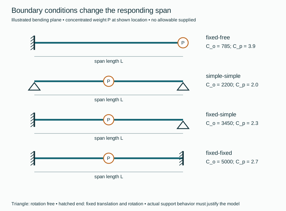
Figure 10.6. Authored semantic diagrams of the four idealizations in Table 10.4. A triangle permits end rotation. A hatched end represents fixed rotation and translation in the illustrated bending plane. The concentrated weight is at the indicated point. Actual support stiffness, gaps and other directions remain separate model inputs. The structured companion records each geometry and coefficient pair.
The method's coefficient is based on empty carbon-steel pipe. Its historical stainless adjustment lowers by 7%. It separately gives a diameter/wall-based water correction curve. Contents and insulation add mass, and a different material or temperature can change stiffness.
Those corrections require their own applicable basis. An unknown weight-table cell is not zero. A curve read is not an exact constant for every filled line.
These estimates do not calculate dynamic stress, damping, local fatigue demand or equipment acceptance. Complex connected spans and real boundary compliance can require a fuller modal model.
Compare the natural response with actual forcing and harmonics. For the described double-acting single-cylinder machine, pulsating-flow frequency is twice shaft speed in revolutions per second.
One adopted equipment criterion requires separation through the fourth forcing harmonic. Another metering-pump guideline proposes natural frequencies much higher than pulsating flow, for example at least five times it.
These bases address different arrangements. Neither equals a universal target of four times shaft speed, nor proves that a chosen support has removed all significant excitation.
Adding a restraint to shift a mode also changes thermal response. Its restrained direction needs evaluation against thermal displacement. A thermal null point in one direction can be useful without being fixed in all directions or all states. When a practical restraint cannot sit at that point, iterate location, flexibility and frequency rather than declare the highest frequency best. Verify the changed operating response and local attachment. The model’s frequency output alone is insufficient.
Preserve the plane, leg lengths and weight convention for a bent span
The straight-span coefficients cannot be carried into a bend merely by adding the leg lengths. Three further idealizations in Figure 10.7 retain both the shape and the direction of bending:
- An equal-leg right-angle span with fixed ends
- A portal with both feet fixed
- An equal-leg stepped span with fixed outer ends
Their concentrated weight is at the indicated location.
For these cases, use the preceding equation with as the individual marked leg length. Use as the total distributed weight of the illustrated span. Thus uniform pipe weight gives for the right angle and for the portal and stepped configurations. This is neither the total developed length nor a straight chord joining the terminals.

Figure 10.7. Conditional empty-carbon-steel frequency idealizations. A–C have equal marked lengths L and the listed concentrated-weight locations. D–E have a short fixed leg , a horizontal leg and an opposite leg . Concentrated weight P is at distance from the lower end of . D permits rotation at that end. E fixes it in the illustrated plane.
All geometry is schematic. In-plane motion lies in the drawn piping plane. Out-of-plane motion is normal to it. Structured configuration and equation data preserve the associations.
Table 10.5. Bent-span coefficients for the stated empty-carbon-steel method and the exact idealizations in Figure 10.7A–C.
| Configuration and weight location |
In-plane |
In-plane |
Out-of-plane |
Out-of-plane |
| A: right angle, P at midpoint of horizontal leg |
3,430 |
0.28 |
830 |
0.28 |
| B: portal, P at midpoint of top leg |
690 |
0.61 |
450 |
0.70 |
| C: stepped span, P at midpoint of vertical leg |
620 |
0.66 |
500 |
0.68 |
The directional coefficients can differ substantially; a brace chosen only from an in-plane response can miss out-of-plane bending.
The unequal three-leg offsets D and E use a separate relation. It applies to in-plane vibration only, with the shortest anchored leg, the horizontal leg and the opposite leg. All lengths, including , are in feet. remains in inches. Write the distributed weight per unit length as in lbf/ft. The dimensionless concentrated-to-short-leg weight ratio and mass-position ratio are:
The shorter leg's distributed weight is used here, not the total weight from the preceding coefficient table. For a uniform pipe section the same weight per length applies to all three legs. The two configuration factors are:
For the matching geometry, the frequency estimate is:
The frequency estimates are in Hz. The entire term in is squared. Changing that grouping or using without multiplying by changes the method. The simple-end and fixed-end configurations retain different factors even when their drawn lengths are identical.
Concentrated-weight position enters through ; moving the same mass along the leg changes its frequency contribution. Saved calculation data and the reproduction script expose the example ratios and denominators.
These coefficients and offset equations start from an empty carbon-steel basis. The method's separate stainless correction and diameter/wall-dependent water correction belong to their stated scope. The offset sheet applies those corrections to its configuration factor. No water-curve value is supplied by this reconstruction, and the retained unknown pipe-weight cells cannot provide or as zero. Use known section and weight data or keep the evaluation incomplete. A different material, temperature, nonuniform section or actual boundary compliance needs its applicable model rather than an unexplained reuse of the coefficients.
The offset guidance also records fatigue failures at the anchored end of the shortest leg in metering-pump service. It proposes restraining axial movement of the horizontal leg as a remedy. That observation identifies the movement path and the local root to investigate. It does not turn a calculated frequency or one added support into general metering-pump acceptance.
An axial restraint changes the configuration for which these equations were written and also changes thermal movement. Reevaluate frequency, excitation, local stress and flexibility for that new configuration instead of continuing to quote the unrestrained estimate. Appurtenance geometry supplies a complementary force-to-section account when measured accelerations and a stiff attachment justify it.
Keep an immersed thermowell's wake separate from the external span
An immersed well is excited by its own crossflow wake. One bounded historical circular-cylinder estimate uses for Reynolds numbers up to . In this estimate, is in ft/s and thermowell diameter is in ft, giving shedding frequency in Hz. The associated guideline compares the well's natural frequency with at least at maximum expected flow. This is a restricted preliminary frequency comparison. It is not a complete thermowell pressure, fatigue, geometry or current standard qualification.
The actual well profile, support and flow range need their qualified evaluation. The external nipple/valve assembly has a different natural response; its span estimate cannot qualify the immersed stem.
Compare the same fatigue quantity over the relevant operating range
Displacement at a point is evidence of response, not a local stress limit. Motion can be small near an anchor while curvature and alternating stress are high. Obtain the measured frequency, direction and amplitude convention with enough spatial and operating-state information to evaluate the relevant span or detail.
The stiff-appurtenance method in Small-bore connections already relates measured acceleration and mass/lever arms to local bending, with phase/sign and separate parent-pipe evaluations. Do not substitute a main-span displacement limit for that evaluation.
A fatigue curve can use stress range while the calculated or measured response uses amplitude. For a symmetric fully reversed sinusoidal stress, . A specifically adopted historical butt-welded carbon-steel atmospheric/noncorrosive basis without significant geometric concentration uses a 9.0-ksi design stress range. On that basis alone, the corresponding amplitude is 4.5 ksi. Its operating-vibration procedure halves the selected design value when only spot observations are available, giving 4.5 ksi of range or 2.25 ksi of amplitude.
The observation factor and range-to-amplitude conversion are separate operations. Neither is a new stress-concentration factor.
These values are not generic endurance limits for every piping weld, stainless or nonmetallic construction, corrosive environment, high temperature or damaged detail. An appropriate local factor and material/detail/environment basis remain necessary. Spot-observation allowance also does not establish that the unobserved worst operating condition is bounded.
Operating integrity retains the observation and response account. The analysis should say whether the operating range was actually monitored and how the selected fatigue basis treats that limitation. Cycle-count time explains urgency but supplies no universal failure life or repair deadline. Structured method and result data keep the numerical examples distinct from project acceptance.
Compare a defined finite-cycle exposure with a compatible design curve
A steady vibration and an infrequent transient can accumulate very different numbers of stress cycles. The historical design curve in Figure 10.8 adds a finite-cycle comparison to the 9.0-ksi endurance-range example above. Its sloping portion permits higher design stress ranges at lower cycle counts, then approaches the stated plateau. It is a design relation with a built-in margin, rather than a measured failure-life curve.
Its scope is full-penetration butt-welded carbon steel in atmospheric, noncorrosive service with no significant geometric stress concentration. A different weld detail, a branch root, corrosion damage or a different material needs its compatible fatigue basis before these ordinates can be used.
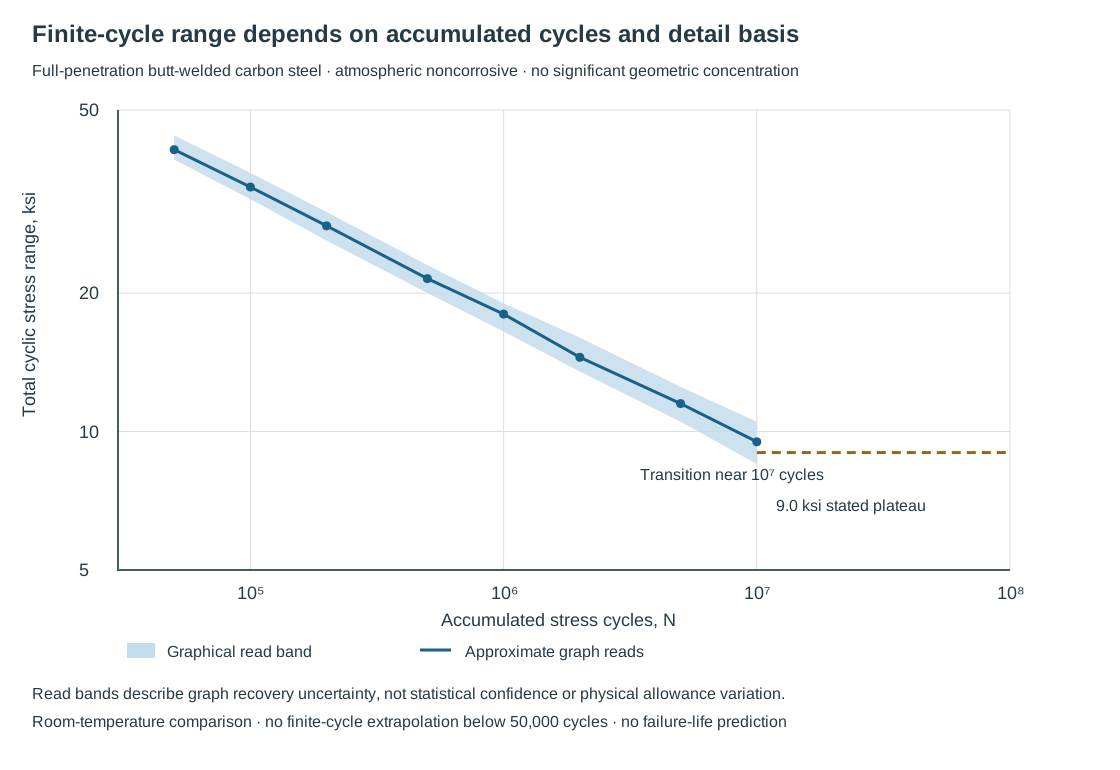
Figure 10.8. A bounded graphical reconstruction on logarithmic axes. Points and the connecting path represent approximate reads over to cycles. The shaded band shows graphical read uncertainty, not statistical confidence or permitted physical variation. The dashed 9.0-ksi line is the separately stated endurance-range level. Its transition occurs around cycles. That cycle count is approximate.
The finite-cycle path is not extrapolated below its recovered range. Structured curve data, calculation data and the reproduction script preserve the inputs and distinctions.
Table 10.6. Approximate total cyclic stress-range ordinates for the stated historical welded-carbon-steel design basis.
| Cycles |
Approximate range, ksi |
Graphical read band, ksi |
| 50,000 |
41 |
39–44 |
| 100,000 |
34 |
32–36.5 |
| 200,000 |
28 |
26–30 |
| 500,000 |
21.5 |
20–23 |
| 1,000,000 |
18 |
16.5–19 |
| 2,000,000 |
14.5 |
13.5–16 |
| 5,000,000 |
11.5 |
10.5–12.5 |
| Around 10,000,000, near the transition |
9.5 |
8.5–10.5 |
These coarse values retain the limits of a plotted curve without inventing exact numerical fatigue coefficients. For an intermediate cycle count within the recovered sloping region, interpolate between adjacent reads in log-cycle and log-stress coordinates. For endpoints and , with a stress range in ksi, the graphical interpolation is:
To retain the read uncertainty:
- Use the same construction for the lower and upper read bands.
- Preserve the resulting interval in the comparison.
This is an interpolation convention for the recovered graph, not an independently established fatigue law. A point whose demand lies inside the read band cannot be settled by displaying more digits from the interpolation.
The evaluated stress must have the same quantity and local-detail basis as the ordinate. For a symmetric fully reversed sinusoidal stress, total range is . Compare demand with the entire read band: below it, above it, or unresolved within it. Such comparison does not predict fracture or grant an operating interval.
For constant-frequency exposure, , with in Hz and in seconds. Repeated constant-frequency bursts can be counted by summing .
Calendar time includes inactive periods and is therefore a different quantity. When stress level or detail changes between intervals, simply adding cycles and comparing the total with one stress ordinate does not establish cumulative fatigue damage. That evaluation needs its own qualified history and damage method. Cycle counts are neither failure predictions nor repair deadlines.
The local stress account remains essential even for a curve with a built-in design margin. Measured displacement, a nominal straight-pipe stress and an intensified branch-root stress are not interchangeable. The evaluation needs the stress location, direction, range/amplitude convention and applicable local factor. A factor already contained in the selected detail assessment must not be counted twice.
A stress concentration cannot be ignored because a pipe's global motion is small. Nor does this butt-weld curve become a general branch or threaded-joint curve by relabeling its ordinate.
Keep temperature and environment local to the decision. The historical discussion treats a room-temperature carbon-steel endurance limit as constant up to 750°F for its purpose, but does not supply a temperature-dependent finite-cycle curve. That endurance statement cannot establish the entire sloping relation at elevated temperature. The finite-cycle comparison here retains a room-temperature, atmospheric, noncorrosive basis. A higher-temperature or aggressive-environment evaluation needs a compatible basis, including the effect of metal loss and changed local stress.
A monitored operating envelope differs from a spot observation. The factor of two described above is specified for design endurance limits when observations may miss the worst condition. It does not supply a separately established finite-cycle curve obtained by halving every ordinate in this table.
A finite-cycle exposure decision needs its stress and cycle history bounded over the relevant operating conditions. One measured amplitude does not provide that history. Use the curve to organize the required comparison and uncertainty. The investigation below establishes the actual motion, operating state, damage condition and remedy.
Investigate the actual operating condition and recheck the remedy
When vibration occurs, record its operating condition:
- Record the equipment running, flow and phase.
- Record the pressure, temperatures, valve positions and transient stage.
To investigate the response:
- Locate the moving spans, attachments and supports.
- Inspect for cracking, looseness, lost contact or damage.
Appropriate measurements describe displacement, velocity or acceleration with frequency, location, direction and amplitude convention. A visual impression without those relationships cannot establish compliance with a numerical vibration criterion.
Separate source correction from response modification. Correcting an unsuitable control-valve application or reducing avoidable cavitation addresses the forcing. Changing a span, adding a restraint, reducing appurtenance mass or altering a support addresses response. For reciprocating equipment, the connected acoustic and mechanical system can require a pulsation study rather than isolated bracing. A remedy must be evaluated under the relevant service and operating range.
A new vibration restraint also affects thermal behavior. Where possible, locate a suitable restraint with little thermal movement in its constrained direction. Then reevaluate flexibility and natural response. If that position is impractical, iterate both evaluations rather than claim that any added steel is an improvement.
Test the changed arrangement in the operating state that produced the problem. Examine the affected details. Suppressed visible movement alone does not prove an existing crack repaired.
Retain the evaluated model, assumptions, geometry, material/temperature data, terminal movements, support characteristics, cases and equipment reactions. Connect them to the actual settings and configuration established in construction and readiness. Operating integrity and Change return observations and altered conditions to that basis. The analysis remains useful when the next participant can identify which physical relationship a change has modified.